Stata? I Only Know Python
Contents
![]()
Stata? I Only Know Python#
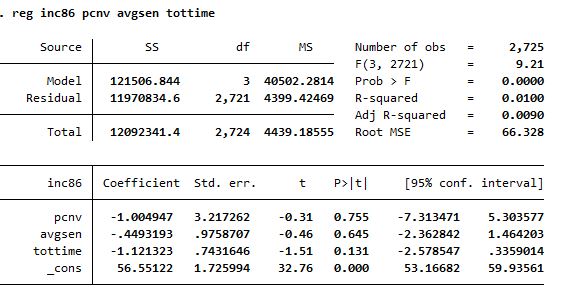
The idea of this class is to mimic the typical output of a Stata least squares regression.Below you can see an example of the output of a regression of this type in Stata using the ‘crime1’ database from the Wooldrige Econometrics book.
Excuting the comand reg inc86 pcnv avgsen tottime the output is:
¡Time To Create!#
As I mentioned before, the idea is to create a class that allows us to replicate Stata output in python. So let’s do it!
# We have to import some modules to use matrix and calculate statistics
import numpy as np
import pandas as pd
import scipy.stats as sst
from scipy import stats

class Lineal_Reg(object):
  def __init__(self,Y,X,alpha=0.05,intercept = True):
    self.intercept = intercept
    self.Y = Y.to_numpy().reshape(len(Y),1)
    if self.intercept == True:
      self.X = np.c_[np.ones(self.Y.shape[0]),X.to_numpy()] if len(X.shape) !=1 else np.c_[np.ones(len(X)),X.to_numpy().reshape([len(X),1])]
    elif self.intercept == False:
      self.X = X.to_numpy() if len(X.shape) !=1 else X.to_numpy().reshape([len(X),1])

    self.alpha = alpha
    self.names = X.columns if len(X.shape)!=1 else [X.name]
    self.n = self.X.shape[0]
    self.k = self.X.shape[1] -1 if len(X.shape) !=1 else 1
    self.gl = self.n - self.k -1

  class fit():
    def __init__(self):
      Lineal_Reg.__init__(self,Y,X,alpha=0.05,intercept = True)
      self.betas = (np.linalg.inv(self.X.T@self.X)@self.X.T@self.Y)

    def __anova(self):
      self.residuals = self.Y - (self.X @ self.betas)
      self.SEC = np.sum(np.square(self.X @ self.betas -np.mean(self.Y)))
      self.SRC = np.sum(np.square(self.residuals))
      self.STC = np.sum(np.square(self.Y-np.mean(self.Y)))
      self.R_2 = 1-self.SRC/self.STC
      self.statistic_F = (self.R_2 / self.k) / ((1-self.R_2)/(self.n - self.k -1))
      self.MS_model = self.SEC / self.k
      self.MS_residual = self.SRC / self.gl
      self.MS_total = self.STC / (self.n - 1)

    def __table_results(self):
      self.m_covariances = (self.SRC/self.gl) * (np.linalg.inv(self.X.T @ self.X))
      self.variances = np.diag(self.m_covariances)
      self.standard_error = np.sqrt(self.variances).ravel().tolist() # ya quedo en lista
      self.t_values = [betas/errors for (betas,errors) in zip(self.betas.ravel().tolist(),self.standard_error)]
      self.p_values = [stats.t.sf(np.abs(t_val), self.n-1)*2 for t_val in self.t_values]  #t,Gl
    #intervals
      self.t_level = sst.t.ppf(1 - self.alpha/2, df=self.n - self.k - 1 )  # df = n-k-1
      self.intervals = [sorted([beta - (errcoef * self.t_level),beta + (errcoef * self.t_level)]) for (beta,errcoef) in zip(self.betas.ravel().tolist(),self.standard_error)]

    @property # decorator to turn a method in an attribute
    def summary(self):
      self.__anova()
      self.__table_results()
      panel = pd.DataFrame(index=['Model','Residuals','Total'])
      panel['SS'] = [round(i,2) for i in [self.SEC,self.SRC,self.STC]]
      panel['df'] = [self.k,self.gl,self.n-1]
      panel['MS'] = [round(i,2) for i in [self.MS_model,self.MS_residual,self.MS_total]]
      panel['  '] = ['   ','   ','   ']
      panel['    '] = [f'No. Observations = {self.n}',f'F{self.k,self.gl} = {round(self.statistic_F,2)}',f'R-squared = {round(self.R_2,4)}']   # Esto toca organizarlo mejor

      results=pd.DataFrame(index= ['_Cons']+ [i for i in self.names]) if self.intercept == True else pd.DataFrame(index= [i for i in self.__names])
      results['Coefficients'] = [round(i,3) for i in self.betas.ravel().tolist()]
      results['S. Error'] = self.standard_error
      results['t'] = [round(i,2) for i in self.t_values]
      results['P'] = [round(i,4) for i in self.p_values]
      results['Confidence Intervals'] = [(round(i[0],6),round(i[1],6)) for i in self.intervals]
      print(panel)
      print()
      print(results)
¡Time To Test!#
Now using the wooldridge python package we can try to execute the same regression model with our class and compare the results
import wooldridge as wd # Dont Forget to install wooldridge package
df = wd.data('crime1')

Y = df['inc86']
X = df[['pcnv','avgsen','tottime']]

model = Lineal_Reg(Y,X,alpha=0.05) # Creating the object
reg = model.fit() # using fit method
reg.summary # Using summary attribute
                    SS    df        MS
Model        121506.84     3  40502.28       No. Observations = 2725
Residuals  11970834.58  2721   4399.42             F(3, 2721) = 9.21
Total      12092341.43  2724   4439.19              R-squared = 0.01

         Coefficients  S. Error      t       P    Confidence Intervals
_Cons          56.551  1.725994  32.76  0.0000  (53.166824, 59.935609)
pcnv           -1.005  3.217262  -0.31  0.7548   (-7.313471, 5.303577)
avgsen         -0.449  0.975871  -0.46  0.6452   (-2.362842, 1.464203)
tottime        -1.121  0.743165  -1.51  0.1315   (-2.578547, 0.335901)
Let’s Talk A Little About What We created …#
The class is mainly composed of two parts, the first is an initiator function __init__() where the first attributes of the object are created and manipulated, which in this case will be the arrays of dependent and independent variables according to the regression. Apart from this initiator function, a class called fit() is created within our first class, the idea is that this is started and the calculation of the betas will be executed, however it is saved and can be accessed using the method converted to summary attribute, which generates all the output with the help of other methods generated within the same subclass. Methods such __anova() and __table_results are hidden to the users, they only work inside the class, we can do thath usgin Methods such __anova() and __table_results are hidden to the users, they only work inside the class, we can do that using __ before the name of a method.
Some Conclusions …#
The main conclusion that stands out from this project is that the open source philosophy and technologies allow us to develop thousands of ideas, codes and applications that some companies would sell. In my case I have the Stata17 license because my university pays for it, however using python I was able to replicate one of the most popular outputs for students of basic econometrics courses.